With recent developments such as Quadtree and Sub-Grid Sampling, TUFLOW opens up the possibilities with regards to accurate modelling of urban environments without the mesh dependency traditionally experienced
13 December 2020
It is estimated that flooding affected over 34 million people and created US$19.7 billion damage globally in 2018 alone (CRED, 2019) and with the impact of climate change and growing populations, flood risk is predicted to increase in many parts of the world (eg Alfieri et al., 2018). Government agencies, whether national or international, and local authorities face a challenging juggling act of protecting people and property with limited budgets. Therefore, flood risk managers utilise benefit-cost ratios to prioritise those areas where there is most benefit to flood risk for the cost of investment in formulating flood risk management strategies. Key to determining the benefit of flood risk is the determination of flood damages particularly in terms of buildings and other property. At the most basic, this requires accurate hydrodynamic modelling of flood depth, which is then used in the calculation of flood damage. The accuracy of the simulated flood depth, and therefore the determination of the impact of flooding is strongly influenced by the hydrodynamic model being used and it's application.
When undertaking hydraulic modelling, one of the primary choices a modeller faces is the discretisation approach used to represent the underlying topography and any geometry that may impact upon the routing of flows. This can be particularly true when simulating flows in urban environments where road networks and buildings can create significant flow routes and obstacles to surface water. The user typically has two choices, a fixed or flexible mesh, both of which have traditionally had their advantages and disadvantages.
Fixed grid/mesh schemes use a regular array of cells of a uniform size, usually squares. Their regular size and shape mean that they are computationally efficient both in terms of memory requirements and run speeds, allowing large domain areas to be simulated quickly. The use of a higher resolution mesh, means that the topographic detail and geometry present in the study area is better represented and intuitively, for a robust 2-dimensional hydrodynamic engine, should lead to a more accurate outputs, for example, flood depths. However, the uniform nature of the grid means that in order to use a small cell size to represent detail that may be present within the study area, the small cell size would have to be used throughout the whole model domain, increasing the amount of memory required, reducing the computational efficiency and increasing the size of the model output files.
As the name suggests, flexible mesh schemes are more flexible in this regard by allowing smaller elements where detail is present within the study area whilst allowing larger mesh elements elsewhere in the model domain thus maintaining simulation efficiency and memory requirements. Typically, triangles and quadrilaterals are utilised. However, this comes at a cost. Flexible meshing requires a meshing algorithm to determine the distribution of mesh elements based on user-defined parameters. Despite automation, generating an accurate and robust mesh which adequately represents the geometry can be a time-consuming activity given the requirement of avoiding thin, poorly shaped elements, and particularly when used in conjunction with mapping data in urban environments. The lack of modeller control over the meshing algorithm very often results in the generation of small elements that require small timesteps to fulfil Courant number requirements and therefore can significantly reduce simulation speeds and lead to much longer simulation times. Increasingly those solvers which do use a flexible mesh are resorting to approaches which allows the meshing algorithm to smooth some of the input geometry to minimise the creation of these small elements. Flexible mesh approaches, on a per cell basis are also less efficient computationally, limiting model sizes and the hydrodynamic calculations are slower.
A recent development in fixed grid modelling is the use of Quadtree schemes that retain the rapid model build and simulation efficiency of fixed grid approaches with the flexibility of the flexible mesh by allowing the variation of cell size within the model domain to represent the detail whilst maintaining computational efficiency.
The 2020 release of TUFLOW saw the addition of such Quadtree functionality. With Quadtree, the cell size can be varied within the model domain allowing for increased resolution down road networks and around buildings as has been shown in previous articles here and here. This is done very quickly and easily using mapping data with minimal setup required. The benefit of the Quadtree approach compared to flexible mesh approaches are three-fold. Firstly, the use of grid cells is more efficient computationally, in terms of data storage, memory requirements and also in terms of hydrodynamic calculations. Secondly, with the Quadtree approach, the cell size, although spatially variable, is user-controlled. As a result, there’s no requirement to assess the mesh for small, poorly shaped elements that bring the required timestep down and therefore significantly impact upon simulation times. If the modeller requires a small cell size to represent particular detail, the modeller can control this. Thirdly, when comparing a modelled option or mitigation scenario to a simulated baseline, with the Quadtree approach, this can be done easily without changing the mesh geometry itself outside of the area of modification. When undertaking a similar assessment with a flexible mesh, adding in further geometric or topographical features to represent an option can result in a different mesh that can, in some instances, change results and make it difficult to determine the impact of the development compared to the baseline scenario.
A further benefit of TUFLOW Quadtree is that it can be used in conjunction with the new Sub-Grid Sampling functionality to allow the representation of solid obstructions such as buildings without needing to align the elements with the building's walls. This means that a fixed grid can now be confidently used at any orientation over an urban area without any need to consider utilising a flexible mesh.
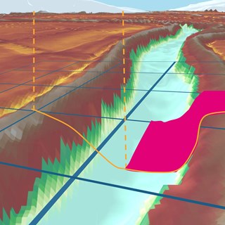
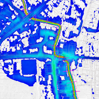
The development of Sub-Grid Sampling (SGS) within TUFLOW allows the full richness of topography data or obstruction outlines (e.g. building footprints) to be utilised regardless of the cell size used within the 2-Dimensional hydrodynamic modelling. The SGS approach and impact is described in the article here and has been demonstrated in the modelling of river channels and whole catchment modelling by Kitts et al. Less, however, has been written regarding it's use in urban areas where the risk of flooding has the greatest impact as it is the interface with people and their properties. Urban environments are challenging environments to simulate, with narrow linear flow paths, rapidly varying topography and barriers to flow such as buildings, particularly when modelling shallow surface water flow. The use of SGS allows the full topographic detail present within any Digital Terrain Model (DTM), or GIS layers of hydraulic obstructions, to be utilised within the hydrodynamic calculations regardless of the cell size, representing road networks, buildings and other obstacles present upon the urban surface.
A key output when assessing surface water flooding is property flood depths, which are often used in conjunction with depth-damage curves to determine property flood damages associated with a particular simulated event, whether it's observed or a design event. These flood depths are often used to support flood risk strategy appraisals to ensure flood risk management is cost effective. It is also an important metric when undertaking flood risk modelling for flood insurance purposes particularly with the growth of parametric insurance.
Figure 1 shows the simulated results for 550 properties when using sub-grid sampling against a traditional approach where a single elevation value is used per cell/element. The simulated flow depths at properties for a range of grid cell sizes have been plotted against the property flow depth at the highest 1m resolution, which is expected to provide the most accurate output of property flow depth. As shown on the top set of graphs, the traditional approach of using one elevation value per cell, without sub-grid sampling, shows the accuracy of the output reducing as the cell size is increased (resolution coarsened). The Y-axis shows the property flood depth for the 1m grid cell size, and the X-axis the property depth when the grid size is varied. The difference between the simulated values for the two cell sizes is shown in the colour of the marker, the darker the colour the closer the correspondence. A trendline and associated correlation coefficient, r, is also displayed to show the strength of the correspondence and the trend. The closer the value to 1, the closer the correlation. As shown in the first few graphs on the top row, when the grid size is small then the results converge as mesh design independency is achieved. As the grid size is increased, the results diverge as shown by the trendline and associated r values. It can clearly be seen that as the cell size increases, the simulated property flood depth reduces, due to the averaging of the underlying topography that takes place by using a larger cell size. The results from the traditional approach when using the 2m and possibly the 5m cell size could be considered sufficiently accurate but the results from the 10m and 20m cell sizes certainly can not be considered creditable and would lead to misleading outcomes.
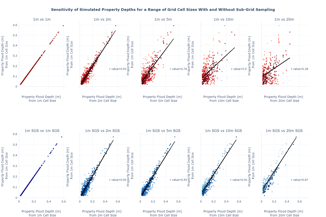
Figure 1: Sensitivity of Simulated Property Flood Depth for a Range of Cell Sizes with the traditional approach to assigning elevations to cells (top set of plots in red) and the sub-grid sampling approach (bottom set of plots in blue). The darker the colour the smaller the difference between the simulated property flood depth and that of a baseline from a 1m cell size (the highest resolution equal to the DTM resolution).
When using SGS the results show much less sensitivity to cell size as shown in the bottom set of graphs. The trendlines and r-squared values suggest that despite the cell size used, there's a good correspondence with the property flood depths with the 1m cell size results. Results are consistent across the 1m, 2m 5m, 10m and, amazingly, even at a 20m cell size.
The key benefit of a larger cell size is a quicker simulation time. Figure 2 shows the simulation speed up versus the simulation time required to simulate the 1m Cell Size model. As can be seen there's over a 30 times speed up when using a 20m cell size and a speed up of 25 and 15 for the 10m and 5m cell sizes respectively.
Obtaining accurate results quicker opens up a host of opportunities in terms of sensitivity testing, uncertainty analysis and the modelling of larger areas. In addition, with such excellent convergence for larger cell sizes, this allows the modeller to operate at a coarser resolution and much faster simulation times during model development, prior to production runs at a finer resolution.
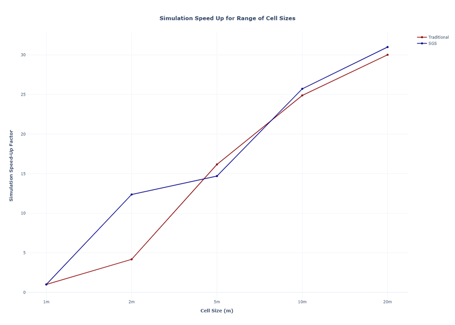
Figure 2: Simulation Speed Ups for a number of cell sizes for a traditional approach and the sub-grid sampling approach.
The importance of the property flood depths can be seen when utilising the property flood depths in conjunction with depth-damage curves to determine the expected flood damage. The flood damage is then used to determine benefit-cost ratios to appraise and support different flood risk management strategies. The simulated property flood depths from Figure 1 were used to calculate expected flood damages and the variation in calculated total property damage with cell size are shown in Figure 3.
The traditional approach to assigning elevations shows significant variation (and therefore loss of accuracy) with the property damages estimated for the larger cell sizes with the 20m cell size being 22% lower than those calculated from 1m cell size outputs. This has the impact of reducing the benefit-cost ratio, potentially mis-representing the benefit, and affecting the chance of obtaining funding for a particular flood risk management strategy.
With the SGS approach the property flood damages calculated based upon the 20m cell size outputs are less than 10% lower than those calculated with the 1m cell size. The standard variation for the calculated property flood damages is also significantly reduced, greatly increasing the consistency of the calculated output regardless of the cell size used.
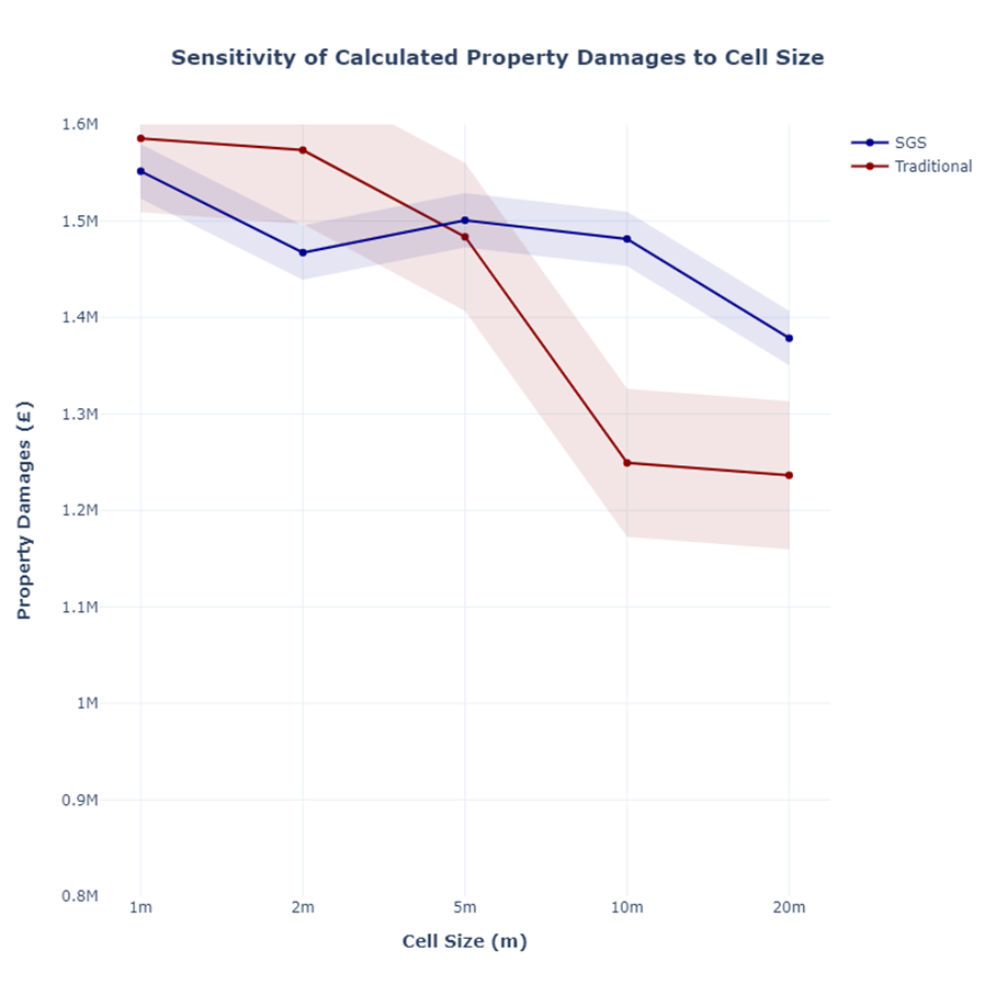
Figure 3: Total Calculated Expected Property Flood Damage for a number of cell sizes for a traditional approach and the sub-grid sampling (SGS) approach.
Flood risk management, and parametric flood insurance, are underpinned by the accuracy of flood depth outputs from hydrodynamic models. It is shown that property flood depths are sensitive to the mesh resolution when using traditional elevation assignment approaches in 2D hydrodynamic models.
Sub-Grid Sampling (SGS) is the process through which all the topographic variation, including hard obstructions such as buildings, at a sub-cell level is utilised within the hydrodynamic calculations regardless of the cell size. It has been observed previously that the approach can eliminate the sensitivity of result outputs to fixed grid mesh orientation and cell size, although this is largely seen with metrics of observed flows and flow velocities. A similar benefit is also seen in surface water flooding of urban environments where SGS can be useful in eliminating result sensitivity to cell size and orientation, removing the need to use flexible meshes or very fine fixed grids around buildings. This has been shown through the sensitivity of property flood depths with cell size that is observed in traditional approaches for assigning elevations for both fixed grids and flexible meshes. Utilising the SGS approach, the flood depths simulated with a 1m cell size can be closely matched and simulated 30-35 times quicker when using a 20m cell size.
The importance of the greater accuracy of property flood depths by utilising SGS can be seen in the consistency of calculated flood damages, an important metric used in flood risk management, across the full range of simulated cell sizes. With the property damages being used to determine benefit cost ratios, or used in parametric flood insurance, it's imperative that accurate damage costs are calculated. This can now be achieved through the use of SGS, removing the need for time-consuming simulations using finer resolutions and sensitivity analysis.
Whilst there is likely to be a middle ground, particularly when mapping hazard which relies on high resolution velocity calculations, the potential for SGS in providing accurate outputs of property flood depths over large model domains at a fraction of the setup time compared with flexible meshes, along with much faster simulation times, is a game-changer for the surface water modelling industry. Where additional detail is required for the mapping of flood hazard or velocity, this can be achieved by utilising the Quadtree approach in areas where high resolution velocity based outputs are needed.
Although this article has focused on property flood depths and damages, there are other scenarios where the consistency of flood depth accuracy across a range of cell sizes is important, including in determining inlet capture rates and determining pump switch-on levels. The wider benefits of using SGS, especially in combination with Quadtree, are considered to be vast.
Alfieri, L., Dottori, F., Betts, R., Salamon, P., and Feyen, L., (2018). Multi-Model Projections of River
Flood Risk in Europe under Global Warming, Climate 6(1).
Centre for Research on the Epidemiology of Disaster (CRED), (2019), Natural Disasters 2018. Brussels.
Kitts, D. Syme, W. Gao, S. Collecutt, G. Ryan, P. 2020. Eliminating Mesh Orientation and Cell Size
Sensitivity in 2D SWE Solvers. Submitted paper for the IAHR 10th Conference on Fluvial Hydraulics,
River Flow 2020, Delft, Netherlands.
TUFLOW - Info
The 2020 release of TUFLOW saw a host of exciting and ground-breaking functionality released. Sub-Grid Sampling, and specifically its applications and its benefits, is the focus of this article.
TUFLOW - Info
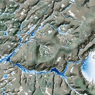
The Pix Brook Flood Study is a multi-stakeholder options and feasibility investigation needing an integrated catchment wide model. TUFLOW was chosen due to its ability to represent surface water, fluvial and pipe networks within the one modelling software.
TUFLOW - Info
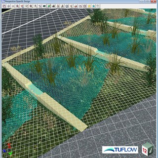
12d Model and TUFLOW provides an excellent way of integrating what were historically siloed areas of responsibility for civil designers, flood modellers and client liaison. This example showcases how 12d Model - TUFLOW can help customers overcome their problems in design and flooding projects by providing the connectivity from concept through to construction.
TUFLOW - Info
TUFLOW CATCH is a new add-on module for both TUFLOW HPC and TUFLOW FV. It enables constituent (e.g. sediment, nutrients, pollutants, pathogens) generation, transport and intervention / mitigation features in the catchment. It also automates boundary condition information transfer between TUFLOW HPC to TUFLOW FV for fully integrated catchment and 3D receiving water modelling. Click here to learn more.